Introduction
This is the second entry in the series on biclustering algorithms, this time covering spectral biclustering. This is the first part, focusing on the Spectral Co-Clustering algorithm (Dhillon, 2001) [1]. The next part will focus on a related algorithm, Spectral Biclustering (Kluger et. al., 2003) [2].
To motivate the spectral biclustering problem, let us return to our friend Bob, who hosted the party in the previous article. Bob is thinking about music again, but this time he is writing song lyrics. Bob plans to imitate popular songs by including similar words in his lyrics. To learn which words to use, he collects the lyrics to many popular songs into a $w \times d$ term frequency matrix $A$, where $A_{ij}$ is the number of times word $i$ appears in song $j$.
Bob knows that his song database contains songs of many different genres. Since the words that are popular in one genre may not be popular in another, he decides to use biclustering again. Bob wants to jointly cluster the rows and columns of $A$ to find subsets of words that are used more frequently in subsets of songs.
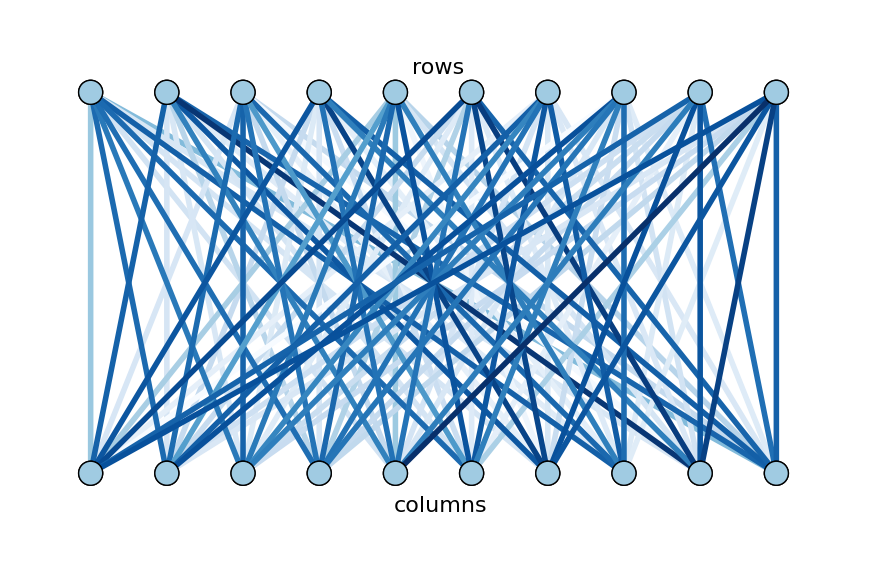
This problem can be converted into a graph partitioning problem: create a graph with $w$ word vertices, $d$ song vertices, and $wd$ edges, each between a song and a word. The edge between song $i$ and word $j$ has weight $A_{ij}$. This graph is bipartite because there are two disjoint sets of vertices (songs and edges) with no edges within sets, and every song is connected to every word. Here is a small example of such a bipartite graph.
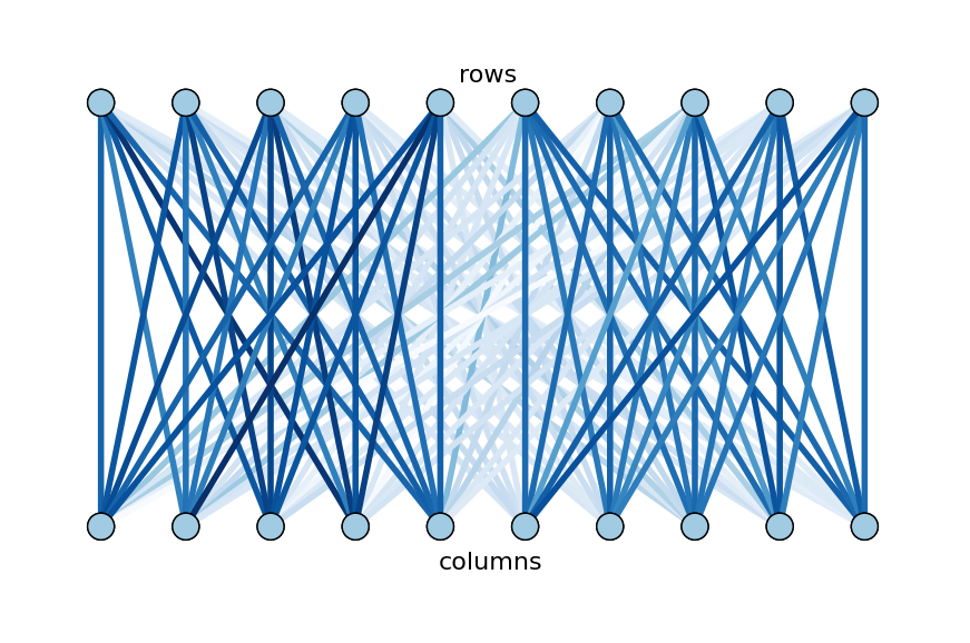
To find biclusters of words and songs, Bob wants to partition the graph so that edges within partitions have heavy weights and edges between partitions have light weights. Furthermore, he would like each partition to be about the same size. This task problem, known as normalized cut, will be formulated more rigorously in the next section. Here is the partitioning of the example graph that achieves Bob’s goal:
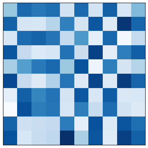
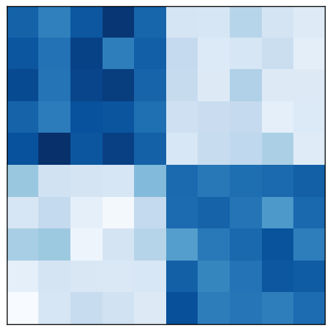
This same data process be visualized as a matrix, too, of course. The original matrix $A$ corresponds to the unpartitioned graph. After rearranging rows and columns, the biclusters corresponding to heavy graph partitions are visible on the diagonal.
The idea of converting a data matrix into a bipartite graph motivates many biclustering algorithms. In this case, the goal of finding the optimal normalized cut leads us to the spectral clustering family of algorithms. Let us see how they work.
Spectral clustering
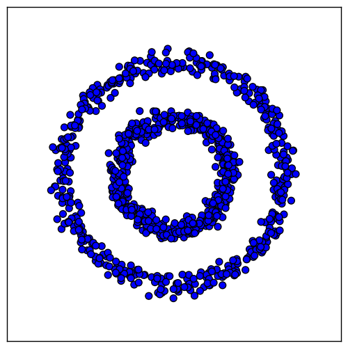
To demonstrate spectral clustering, we will use a toy dataset consisting of two-dimensional data points that form concentric rings:
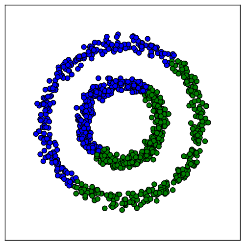
We would like the samples within each ring to cluster together. However, algorithms like k-means will not work, because samples in different rings are closer to each other than samples in the same ring. It might lead, for example, to this result:
Spectral clustering will allow us to convert this data to a new space in which k-means gives better results. To find this new space, we start by building a graph $G = \{ V, E \}$ with a vertex for each sample. Each pair of samples $x_i, x_j$ is connected by an edge with weight $s(x_i, x_j)$ equal to the similarity between them. The goal when building $G$ is to capture the local neighborhood relationships in the data. For simplicity, we achieve this goal by setting $s(x_i, x_j) = 0$ for all but the nearest neighbors.
Let square matrix $W$ be the weighted adjacency matrix for $G$, so that $W_{ij}=s(x_i, x_j)$ when $i \neq j$ and $W_{i, i} = 0$. Let $D$ be the degree matrix for $G$, which is a diagonal matrix containing the sum of all weights for edges incident to vertex $i$: $D_{i, i} = \sum_{j=1}^{n} W_{ij}$, and $D_{i, j}=0$ if $i \ne j$. Then the Laplacian matrix of graph $G$ is defined as $L=D-W$. The Laplacian is used in many graph problems because of its useful properties. For this problem we will use the following property: the smallest eigenvalue of $L$ is 0, with eigenvector $\mathbb{1}$.
To see why this property is useful, consider the ring problem again. In this particular case, we were lucky when building graph $G$, because it contains two connected components, each corresponding to one of the clusters we would like to find. The Laplacian makes it easy to recover those clusters. Since there are no edges between components, $W$ is block diagonal, and therefore $L$ is block diagonal. Each block of $L$ is the Laplacian for a connected component. In this case, since the two submatrices $L_1$ and $L_2$ are also Laplacians, they each have eigenvalues of 0 and eigenvectors of $\mathbb{1}$. Therefore, we know that the eigenvalue 0 of $L$ has multiplicity two, and its eigenspace is spanned by $[0, \dots , 0, 1, \dots , 1]^\top$ and $[1, \dots , 1, 0, \dots , 0]^\top$, where the number of $1$ entries in each vector is equal to the number of vertices in that connected component.
This realization suggests a strategy for finding $k$ clusters if they appear in the graph as connected components:
Build graph $G$ and compute its Laplacian $L$.
Compute the first $k$ eigenvectors of $L$.
The nonzero entries of eigenvector $u_i$ indicate the samples belonging to cluster $i$.
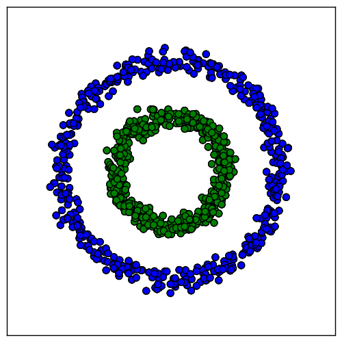
Applying this method to the circles dataset does indeed locate the correct clusters:
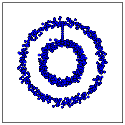
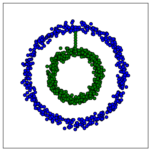
Unfortunately, most of the time $G$ will not be so conveniently separated into connected components. For instance, if we add a bridge between the rings, the resulting graph has only one connected component, even with the nearest-neighbor affinities:
We can deal with this case by removing a few edges to create two connected components again. To do so, we introduce the notion of a graph cut. The following definition will be needed: if $V_i$ and $V_j$ are sets of vertices,
$$W(V_i) = \sum_{a, b \in V_i, a \neq b} W_{ab}$$
is the sum of edge weights within a partition and
$$W(V_i, V_j) = \sum_{a \in V_i, b \in V_j} W_{ab}$$
is the sum of edge weights between the two partitions. Then given a partition of the set of vertices $V = V_1 \cup V_2 \dots \cup V_k$,
$$\text{cut}(V_1 \dots V_n) = \frac{1}{2} \sum_{i=1}^k W(V_i, \overline{V_i})$$
where $\overline{V_i}$ denotes the complement of $V_i$. The factor of $\frac{1}{2}$ corrects for double counting.
We want to partition the graph to minimize the cut, but the minimum is trivially achieved by setting one $V_i = V$ and $V_j = \emptyset$ for $i \neq j$. To ensure that each partition is approximately balanced, we instead minimize the normalized cut, which normalizes by the weight of each partition:
$$\text{ncut}(V_1 \dots V_n) = \sum_{i=1}^k \frac{\text{cut}(V_i, \overline{V_i})}{W(V_i)}$$
There are other balanced cuts, such as ratio cut, but here we focus on normalized cut because it will be used again in the Spectral Co-Clustering algorithm.
Unfortunately, the normalized cut problem is in NP-hard. However, the relaxed version of this integer optimization problem can be solved efficiently. Moreover, it turns out that the first $k$ eigenvectors of the generalized eigenproblem $Lu = \lambda D u$ provide the solution to the relaxed problem. This real solution can then be converted into a (potentially suboptimal) integer solution by a clustering; here we will use k-means.
The steps for spectral clustering, minimizing $\text{ncut}$, are:
Build graph $G$ and compute its Laplacian $L$.
Compute the first $k$ eigenvectors of $Lu = \lambda D u$.
Treat the eigenvectors as a new data set with $n$ samples and $k$ feature. Use k-means to cluster it.
In our ring problem, the optimal normalized cut is the one that cuts through the bridge. The solution found by spectral clustering is the optimal one:
The properties of the graph Laplacian are what make this method work. The first $k$ eigenvectors provide an alternative representation of the data in a space in which it is more amenable to clustering by algorithms such as k-means.
This section gave a simplified introduction to spectral clustering on a toy example. Hopefully it has provided the reader with some intuition for how these methods work. However, it has necessarily skipped many important details. For a more complete overview, see [3], from which this section has been adapted.
Spectral Co-Clustering
Let us return to Bob’s songwriting to see how our new insights can be applied to his problem. Remember that Bob had converted his word frequency matrix into a bipartite graph $G$. Remember also that he wants to partition it into $k$ partitions by finding the optimal normalized cut. We saw in the previous section how to find a solution to this problem, which involved finding the eigenvectors of the matrix $L$. We could do that directly here, too, but we can avoid working on the $(w+d) \times (w+d)$ matrix $L$ and instead work with the smaller $w \times d$ matrix $A$.
If we normalize $A$ to $A_n$ in a particular way, the singular value decomposition of the resulting matrix $A_n = U \Sigma V^\top$ will give us the desired partitions of the rows and columns of $A$. A subset of the left singular vectors will give the word partitions, and a subset of the right singular vectors will give the song partitions.
The normalization is performed as follows:
$$A_n = R^{−1/2} A C^{−1/2}$$
Where $R$ is the diagonal matrix with entry $i$ equal to $\sum_{j} A_{ij}$ and $C$ is the diagonal matrix with entry $j$ equal to $\sum_{i} A_{ij}$.
If $k=2$, we can use the singular vectors $u_2$ and $v_2$ ($u_1$ and $v_1$ are discarded) to compute the second eigenvector of $L$:
$$z_2 = \begin{bmatrix} R^{-\frac{1}{2}} u_2 \\\ C^{-\frac{1}{2}} v_2 \end{bmatrix}$$
We know how to proceed from here: as we saw in the previous section, clustering this eigenvector provides the desired bipartitioning.
If $k>2$, then the $\ell = \lceil \log_2 k \rceil$ singular vectors, starting from the second, provide the desired partitioning information. In this case, we cluster the matrix $Z$:
$$Z = \begin{bmatrix} R^{-\frac{1}{2}} U \\\ C^{-\frac{1}{2}} V \end{bmatrix}$$
where the columns of $U$ are $u_2, \dots, u_{\ell + 1}$, and similarly for $V$.
Here is full algorithm for finding $k$ clusters, adapted from the original paper:
Given $A$, normalize it to $A_n = R^{-\frac{1}{2}} A C^{-\frac{1}{2}}$.
Compute $\ell = \lceil \log_2 k \rceil$ singular vectors of $A_n$, $u_2 \dots u_{\ell+1}$ and $v_2 \dots v_{\ell+1}$. Form the matrix $Z$ as just shown.
Cluster with k-means the $\ell$-dimensional data $Z$ to obtain the desired $k$ biclusters.
Notice that the $w$ rows and $d$ columns of the original data matrix are converted to the $w+d$ rows in matrix $Z$. Therefore, both rows and columns are treated as samples and clustered together.
Example: clustering documents and words
To see the algorithm in action, let us try clustering some documents.
from sklearn.feature_extraction.text import TfidfVectorizer
from sklearn.cluster.bicluster import SpectralCoclustering
import requests
import time

url_base = "http://www.gutenberg.org/cache/epub/{0}/pg{0}.txt"
ids = [1228, 22728, 5273, 19192, 2926, 2929, 6475, 20818, 24648,
       22428, 35937, 27477, 6630, 15636, 35744, 26556, 6574, 28247,
       25992, 28613]
docs = []
for i in ids:
    docs.append(requests.get(url_base.format(i)).text)
    time.sleep(30)  # be nice to the server

vec = TfidfVectorizer(stop_words='english')
model = SpectralCoclustering(n_clusters=2, svd_method='arpack')
data = vec.fit_transform(docs).T
model.fit(data)
In this example, we download twenty books from Project Gutenberg, ten
from the astronomy category and ten from the evolution category. The
word frequency matrix is created with
tf-idf values. The
dataset is a $38,121 \times 20$ sparse scipy matrix. The
SpectralCoclustering model supports sparse matrices, so we can pass
it directly. The biclustering step took 0.4 seconds on a laptop with a
Core i5-2520M processor.
To examine whether the biclusters are reasonable, we determine the most important words in each bicluster by subtracting the sum of frequencies outside the bicluster from the sum of frequencies within the bicluster. The first bicluster contained thirteen documents, of which eight were on astronomy. The most important words in this bicluster were “et”, “copernican”, “bruno”, “paris”, “speech”, “congregation”, “acid”, “1616”, “scriptures”, and “ii”. The other bicluster contained the remaining documents, with the following important words: “species”, “selection”, “case”, “different”, “number”, “darwin”, “characters”, “size”, “genera”, and “conditions”. These seem like reasonable words to find in old texts on astronomy and evolution, respectively.
The functionality demonstrated in this section will eventually be available in scikit-learn. In the meantime, if you would like to try the code, check out my personal branch.
Conclusion
This article introduced spectral clustering. It then demonstrated how the same method was adapted to biclustering in the Spectral Co-Clustering algorithm. We have seen how the algorithms work on toy datasets. Finally, we saw how to use scikit-learn to bicluster a more realistic dataset.
The next post, part two of this series, will continue the discussion of spectral methods. It will introduce a new type of bicluster, the checkerboard structure, and a new algorithm for finding checkerboard patterns, the Spectral Biclustering algorithm (Kluger, 2003).
References
[1] Dhillon, I. S. (2001, August). Co-clustering documents and words using bipartite spectral graph partitioning. In Proceedings of the seventh ACM SIGKDD international conference on Knowledge discovery and data mining (pp. 269-274). ACM.
[2] Kluger, Y., Basri, R., Chang, J. T., & Gerstein, M. (2003). Spectral biclustering of microarray data: coclustering genes and conditions. Genome research, 13(4), 703-716.
[3] Von Luxburg, U. (2007). A tutorial on spectral clustering. Statistics and computing, 17(4), 395-416.