Introduction
The subject of today’s post is a biclustering algorithm commonly referred to by the names of its authors, Yizong Cheng and George Church [1]. It is one of the best-known biclustering algorithms, with over 1,400 citations, because it was the first to apply biclustering to gene microarray data. This algorithm remains popular as a benchmark: almost every new published biclustering algorithm includes a comparison with it.
Cheng and Church were interested in finding biclusters with a small mean squared residue, which is a measure of bicluster homogeneity. To define the mean squared residue, the following notation will be necessary: let $A$ be a matrix, and let the tuple $(I, J)$ represent a bicluster of $A$, where $I$ is the set of rows in the bicluster, and $J$ is the set of columns. The submatrix of $A$ defined by this bicluster is $A_{I J}$. Let $a_{ij}$ with $i \in I, j \in J$ be an element of the bicluster, and let
$$a_{iJ} = \frac{1}{|J|} \sum_{j} a_{ij}$$
$$a_{Ij} = \frac{1}{|I|} \sum_{i} a_{ij}$$
$$a_{I J} = \frac{1}{|I| |J|} \sum_{i, j} a_{ij}$$
be the row, column, and overall means of the bicluster. Then the residue of element $a_{ij}$ is
$$a_{ij} - a_{i J} - a_{I j} + a_{I J}$$
and the mean squared residue of the bicluster is
$$H(I, J) = \frac{1}{|I| |J|} \sum_{i \in I, j \in J} \left (a_{ij} - a_{iJ} - a_{Ij} + a_{I J} \right )^2$$
The residue is meant to measure how an element differs from the row mean, column mean, and overall mean of the bicluster. If all the elements of the bicluster have small residues, clearly the mean squared residue will be small.
$H(I, J)$ achieves a minimum when all the rows and columns of the bicluster are shifted versions of each other. In other words, if we can represent every element of the bicluster as $a_{ij} = r_i + c_j$, where $r$ is a column vector with $|I|$ entries and $c$ is a row vector with $|J|$ entries, then the score of $M$ will be 0.
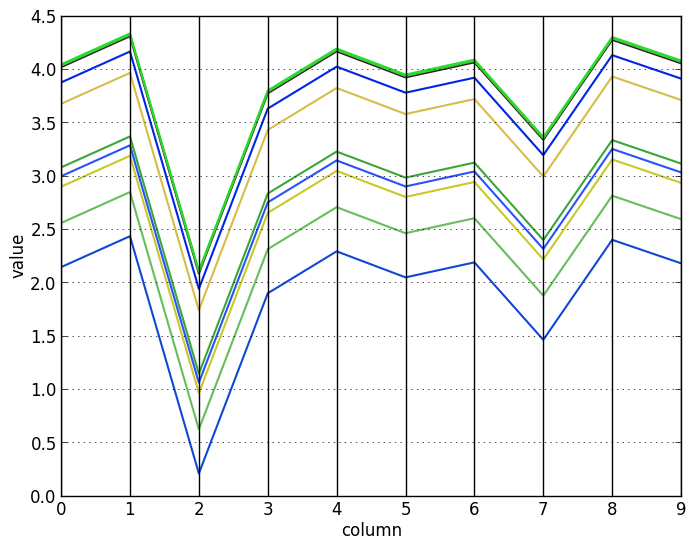
To visualize these shifted rows and columns, here is a matrix with a perfect mean squared residue:
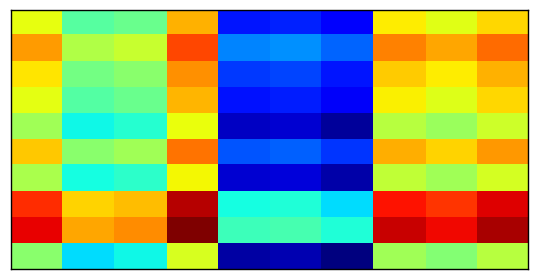
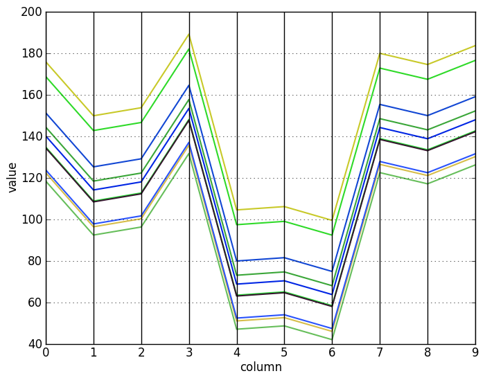
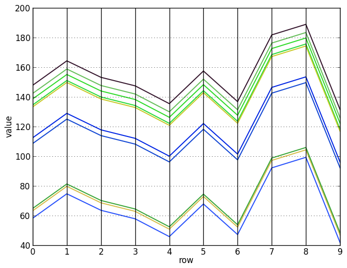
Visualizing the rows and columns of this matrix with a parallel coordinates plot makes the pattern much easier to see. Now it is clear that the row vectors differ from each other by only an additive constant (top), and similarly for the column vectors (bottom):
As a corollary, it is easy to see that there are some special cases: constant biclusters, biclusters with identical rows or columns, and biclusters with only one row or column clearly have a score of 0. Also, it is clear that shifting $A_{I J}$ to $A_{I J} + c$ for any constant $c$ does not change its score.
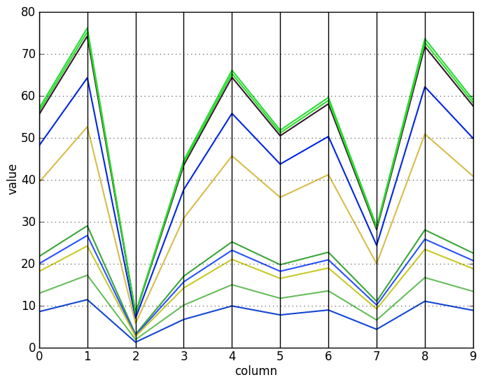
Another corollary is that if the rows and columns of a bicluster are scaled versions of each other, log-transforming the bicluster makes its $H$ score 0. In other words, if $u$ and $v$ are any column vectors, the $H$ score of $u v^\top$ may be large, but the $H$ score of $\log(u v^\top)$ is 0. Therefore, Cheng and Church can also find biclusters with scaling patterns, if the dataset is first log-transformed.
To visualize the effect of the log-transformation, here are some scaled vectors (top) and the same vectors after log-transforming them (bottom):
Let us now see how to find these kinds of biclusters.
The algorithm
Cheng and Church tries to find biclusters that are as large as possible, with the restriction that their $H$ score must be less than some threshold $\delta$. Like most biclustering problems, this one is NP-hard. Therefore, the method proceeds via a simple greedy approach: it starts with the largest possible bicluster, then removes rows and columns that most reduce $H(I, J)$.
As Cheng and Church prove in their paper, this greedy removal can be done efficiently, without the need to recalculate $H$ for every possible row and column removal. To do so, we define the mean squared residue of any row $i$ or any column $j$ in the bicluster as:
$$d(i) = \frac{1}{|J|} \sum_{j \in J} \left (a_{ij} - a_{iJ} - a_{Ij} + a_{I J} \right )^2$$
$$d(j) = \frac{1}{|I|} \sum_{i \in I} \left (a_{ij} - a_{iJ} - a_{Ij} + a_{I J} \right )^2$$
Then this part of the algorithm, the single node deletion step, proceeds as follows:
**Algorithm**: node deletion
**input**: matrix $A$, row set $I$, column set $J$, $\delta>=0$
**output**: row set $I'$ and column set $J'$ so that $H(I', J') <= \delta$
**while** $H(I, J) > \delta$:
    find the row $r = \mathop{\arg\max}\limits\_{i \in I} d(i)$ and the column $c = \mathop{\arg\max}\limits\_{j \in J} d(j)$
    **if** $d(r) > d(c)$ **then** remove $r$ from $I$ **else** remove $c$ from $J$
**return** $I$ and $J$
In order to speed up node deletion, Cheng and Church also uses a method to remove multiple rows and columns at once. This multiple node deletion step proceeds as follows:
**Algorithm**: multiple node deletion
**input**: matrix $A$, row set $I$, column set $J$, $\delta>=0$, $\alpha > 0$
**output**: row set $I'$ and column set $J'$ so that $H(I', J') <= \delta$
**while** $H(I, J) > \delta$:
    remove from $I$ all rows with $d(i) > \alpha H(I, J)$
    remove from $J$ all columns with $d(j) > \alpha H(I, J)$
    **if** $I$ and $J$ have not changed **then** switch to single node deletion
**return** $I$ and $J$
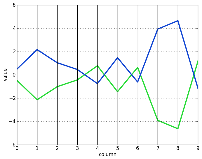
Multiple and single node deletion stop when $H(I, J) <= \delta$. At this point, the algorithm tries a node addition step to add any rows or columns that do not make $H(I, J)$ worse. This step optionally also adds rows if their inverses match the pattern of the bicluster. In the context of microarray data, such rows represent genes with the same, but opposite, regulation patterns. The following two vectors, each the inverse of the other, demonstrates this concept:
The node addition algorithm proceeds as follows:
**Algorithm**: node addition
**input**: matrix $A$, row set $I$, column set $J$
**output**: row set $I'$ and column set $J'$ so that $H(I', J') <= H(I, J)$
**iterate**:
    compute $a\_{i J}$ for all $i$, $a\_{I j}$ for all $j$, $a\_{I J}$, and $H(I, J)$
    add to $J$ any column $j \notin J$ with $\frac{1}{|I|} \sum\_{i \in I} \left (a\_{ij} - a\_{iJ} - a\_{Ij} + a\_{I J} \right )^2 <= H(I, J)$
    recompute $a\_{i J}$, $a\_{I J}$, and $H(I, J)$
    add to $I$ any row $i \notin I$ with $\frac{1}{|J|} \sum\_{j \in J} \left (a\_{ij} - a\_{iJ} - a\_{Ij} + a\_{I J} \right )^2 <= H(I, J)$
    add to $I$ any row $i \notin I$ with $\frac{1}{|J|} \sum\_{j \in J} \left (-a\_{ij} + a\_{iJ} - a\_{Ij} + a\_{I J} \right )^2 <= H(I, J)$
    **if** $I$ and $J$ have not changed **then** break
**return** $I$ and $J$
After node addition, the bicluster is added to the list of results and the algorithm starts again from the beginning. However, because this is a deterministic procedure, it would just find the same bicluster again. Therefore, after finding a bicluster, its entries in the original data are replaced by entries drawn from a uniform random distribution over the range determined by the minimum and maximum of the original dataset.
The whole algorithm looks like this:
**Algorithm**: Cheng and Church
**input**: matrix $A$, number of clusters $N$, $\delta>=0$, $\alpha > 0$
**output**: a set of $N$ biclusters, each with $H(I, J) <= \delta$
**for** $i \leftarrow 1 \dots N$:
    initialize $(I, J)$ to all rows and all columns
     multiple node deletion
     single node deletion
     node addition
     append $(I, J)$ to results
     mask $A\_{I J}$ with random entries
**return** results
Now that we understand how the algorithm works, let us see it in action.
Example
I have implemented Cheng and Church for scikit-learn. To see it in action, we cluster the same lymphoma/leukemia dataset [2] clustered in the original paper and available at the supplementary information page. The data has shape $4096 \times 96$. The parameters used for Cheng and Church were taken directly from the paper.
import urllib
import numpy as np
from pandas import DataFrame
from pandas.tools.plotting import parallel_coordinates
import matplotlib.pylab as plt
from sklearn.cluster.bicluster import ChengChurch

# get data
url = "http://arep.med.harvard.edu/biclustering/lymphoma.matrix"
lines = urllib.urlopen(url).read().strip().split('\n')
# insert a space before all negative signs
lines = list(' -'.join(line.split('-')).split(' ') for line in lines)
lines = list(list(int(i) for i in line if i) for line in lines)
data = np.array(lines)

# replace missing values, just as in the paper
generator = np.random.RandomState(0)
idx = np.where(data == 999)
data[idx] = generator.randint(-800, 801, len(idx[0]))

# cluster with same parameters as original paper
model = ChengChurch(n_clusters=100, max_msr=1200,
                    deletion_threshold=1.2, inverse_rows=True,
                    random_state=0)
model.fit(data)

# find bicluster with smallest msr and plot it
msr = lambda a: (np.power(a - a.mean(axis=1, keepdims=True) -
                          a.mean(axis=0) + a.mean(), 2).mean())
msrs = list(msr(model.get_submatrix(i, data)) for i in range(100))
arr = model.get_submatrix(np.argmin(msrs), data)
df = DataFrame(arr)
df['row'] = map(str, range(arr.shape[0]))
parallel_coordinates(df, 'row', linewidth=1.5)
plt.xlabel('column')
plt.ylabel('expression level')
plt.gca().legend_ = None
plt.show()
The biclustering step took 33.9 seconds on a laptop with a Core i5-2520M processor.
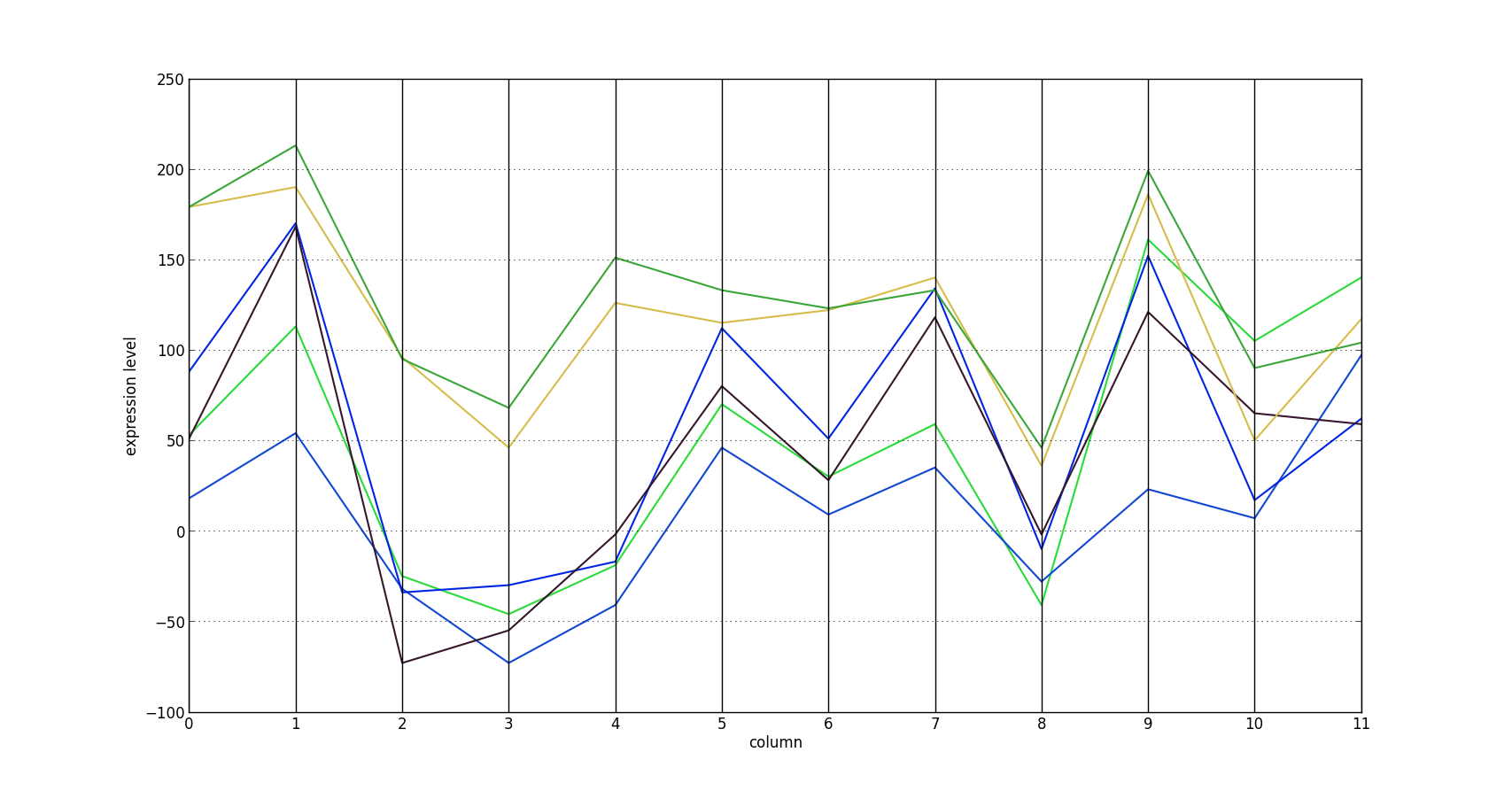
By visualizing the parallel coordinates plot of the bicluster with the smallest $H$ score, it is easy to see that its rows are approximately shifted versions of each other. Each of the six rows represents the expression profile of a gene. This bicluster has an $H$ score of 853.14.
This functionality is not yet merged into scikit-learn. Until it is, check out my personal branch.
Conclusion
We have defined the mean squared residue, which is used to find biclusters with additive shift patterns in their rows and columns. We have seen how Cheng and Church works, and seen how to use the version implemented in scikit-learn.
Though subsequent algorithms have improved on it in various ways, Cheng and Church remains a popular benchmarking method. The next post will cover BiMax, a simple algorithm designed specifically for benchmarking that nevertheless gets good results.
References
[1] Cheng, Y., & Church, G. M. (2000, August). Biclustering of expression data. In Ismb (Vol. 8, pp. 93-103).
[2] Alizadeh, A. A., Eisen, M. B., Davis, R. E., Ma, C., Lossos, I. S., Rosenwald, A., … & Staudt, L. M. (2000). Distinct types of diffuse large B-cell lymphoma identified by gene expression profiling. Nature, 403(6769), 503-511.