Introduction
Continuing the series on biclustering algorithms, this post is about BiMax, a method developed to serve as a baseline in a comparison of biclustering algorithms [1]. Because BiMax was developed as a reference method, its objective is intentionally simple: it finds all biclusters consisting entirely of 1s in a binary matrix.
Specifically, BiMax enumerates all inclusion-maximal biclusters, which are biclusters of all 1s to which no row or column can be added without introducing 0s. More formally, an inclusion-maximal bicluster of $m \times n$ binary matrix $M$ is a set of rows and a set of columns $(R, C)$, with $R \in 2^{\{1, \dots, m \}}$ and $C \in 2^{\{1, \dots, n\}}$ such that:
$\forall i \in R, \forall j \in C : M[i, j] = 1$
for any other bicluster $(R’, C’)$ that meets the first condition, $(R \subseteq R’ \land C \subseteq C’) \implies (R = R’ \land C = C’)$
BiMax only works with binary matrices, but of course non-binary data can be converted to binary data in a number of ways. The simplest method is to threshold it at some threshold $t$, where $t$ could be the mean, median, some other quantile, or any arbitrary threshold. Of course, more sophisticated binarizing methods may also be used.
Now let us see how the algorithm works.
Method
BiMax uses a recursive divide and conquer strategy to enumerate all the biclusters in a $m \times n$ matrix $M$. To illustrate the process we will use the following data matrix, taken from the original paper:
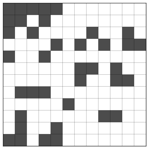
The process begins by choosing any row containing a mixture of 0s and 1s. In this case, all the rows fits this criterion. (If no such row exists, then clearly either all entries of $M$ are 1, in which case the entire matrix is a single bicluster, or all its entries are 0, in which case it has no biclusters.) We arbitrarily choose the first row. The chosen row $r^*$ will be used to divide $M$ into two submatrices, each of which can be processed independently.
To find this submatrices, first the columns $C = \{1, \dots, n\}$ are divided into two sets: those for which row $r^*$ is 1, and those for which it is 0.
- $C_U = \{c : M[r^*, c] = 1\}$
- $C_V = C - C_U$
Next the $m$ rows of $M$ are divided into three sets:
- $R_U$: rows with 1s only in $C_U$
- $R_W$: rows with 1s in both $C_U$ and $C_V$
- $R_V$: rows with 1s only in $C_V$
After rearranging the rows and columns of $M$ to make each set contiguous, the matrix looks like this:
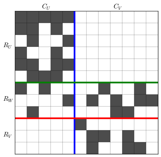
This image makes it clear how to divide the matrix for the recursive step. The submatrix formed by $(R_U, C_V)$ is empty and cannot contain any biclusters. The submatrix $U = (R_U \cup R_W, C_U)$, shown in blue in the next figure, and the submatrix $V = (R_W \cup R_V, C_U \cup C_V)$, shown in red, contain all possible biclusters in $M$. The procedure continues by recursively processing $U$ and then $V$.
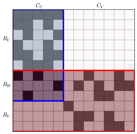
There is one problem yet to address: because $U$ and $V$ overlap, it is possible that a bicluster in $U$ has some rows in $V$. Then that part of the bicluster would be a maximal bicluster in $V$ but not in $M$. To avoid this error, BiMax requires that any bicluster found in $V$ must contain at least one column from each column set in $Z$, where $Z$ is the set of all $C_V$ column sets in the current call stack.
The full algorithm is available in the paper’s supplementary material.
Example
I have implemented the BiMax algorithm in Python. However, even after optimizing it and rewriting parts in Cython, mine is so much slower than the original implementation that it will probably not be added to scikit-learn. For now I have made the pure Python version available.
Here is a simple example of BiMax in action. Since the pure Python version is slow, here we demonstrate it with a small artificial dataset.
import numpy as np
from matplotlib import pyplot as plt
from bimax import BiMax

generator = np.random.RandomState(1)
data = generator.binomial(1, 0.5, (20, 20))

model = BiMax()
model.fit(data)

# get largest bicluster
idx = np.argmax(list(model.rows_[i].sum() * model.columns_[i].sum()
                     for i in range(len(model.rows_))))
bc = np.outer(model.rows_[idx], model.columns_[idx])

# plot data and overlay largest bicluster
plt.pcolor(data, cmap=plt.cm.Greys, shading='faceted')
plt.pcolor(bc, cmap=plt.cm.Greys, alpha=0.7, shading='faceted')
plt.axis('scaled')
plt.xticks([])
plt.yticks([])
plt.savefig('../../images/bimax_example.png', bbox_inches='tight')
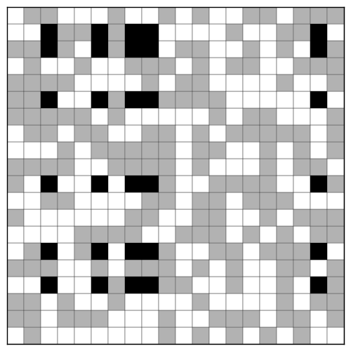
Here is the resulting image, with the original data in gray and the largest bicluster highlighted in black:
Conclusion
This post showed how BiMax works and demonstrated its use. It interesting to note that BiMax’s objective is equivalent to finding all bicliques in the bipartite graph representation of the binary matrix. A recent meeting abstract by Voggenreiter, et. al, in BMC Bioinformatics describes a variant of the Bron-Kerbosch algorithm for enumerating bicliques that in their tests was faster than BiMax.
References
[1] Prelić, A., Bleuler, S., Zimmermann, P., Wille, A., Bühlmann, P., Gruissem, W., … & Zitzler, E. (2006). A systematic comparison and evaluation of biclustering methods for gene expression data. Bioinformatics, 22(9), 1122-1129.